import numpy as np
import pandas as pd
import seaborn as sns
import matplotlib.pyplot as plt
# import warnings
import warnings
# filter warnings
warnings.filterwarnings('ignore')
train = pd.read_csv('/content/drive/MyDrive/military/mnist/train.csv')
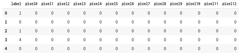
print(train.shape)
train.head()
'''
결과1
'''
# put labels into y_train variable
Y_train = train['label']
# Drop 'label' column
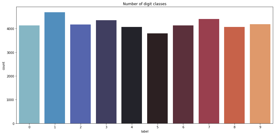
X_train = train.drop(labels=['label'], axis=1)# visualize number of digits classes
plt.figure(figsize=(15, 7))
g = sns.countplot(Y_train, palette='icefire')
plt.title("Number of digit classes")
Y_train.value_counts()
'''
1 4684
7 4401
3 4351
9 4188
2 4177
6 4137
0 4132
4 4072
8 4063
5 3795
Name: label, dtype: int64
'''
'''
결과2
'''
seaborn.countplot(x=None, y=None, hue=None, data=None, order=None, hue_order=None,
orient=None, color=None, palette=None, saturation=0.75, dodge=True, ax=None, **kwargs)
import seaborn as sns
sns.set_theme(style='darkgrid')
ax = sns.countplot(x=Y_train)
'''결과1-1'''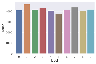
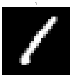
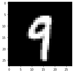
# plot some samples
img = X_train.iloc[0].values
img = img.reshape((28, 28))
plt.imshow(img, cmap='gray')
plt.title(train.iloc[0, 0])
plt.axis('off')
plt.show()
'''
결과3
'''
matplotlib.pyplot.imshow(X, cmap=None, norm=None, *, aspect=None, interpolation=None, alpha=None,
vmin=None, vmax=None, origin=None, extent=None, interpolation_stage=None, filternorm=True,
filterrad=4.0, resample=None, url=None, data=None, **kwargs)
X: array-like or PIL image
shape are (M, N), (M, N, 3), (M, N, 4)
cmap: str ror Colormap
# Normalize the data
X_train = X_train/255.0 # 흑백 색상의 최대 크기로 나눔
print("X_train shape", X_train.shape)
'''
X_train shape (42000, 784)
'''
# Reshape
X_train = X_train.values.reshape(-1, 28, 28, 1)
print("X_train shape:", X_train.shape)
'''
X_train shape: (42000, 28, 28, 1)
'''# Label Encoding
from keras.utils.np_utils import to_categorical # convert to one-hot-encoding
Y_train = to_categorical(Y_train, num_classes=10)tf.keras.utils.to_categorical(
y, num_classes=None, dtype='float32'
)# split the train and the validation set for the fitting
from sklearn.model_selection import train_test_split
X_train, X_val, Y_train, Y_val = train_test_split(X_train, Y_train, test_size=0.1, random_state=2)
print(X_train.shape)
print(X_val.shape)
print(Y_train.shape)
print(Y_val.shape)
'''
(37800, 28, 28, 1)
(4200, 28, 28, 1)
(37800, 10)
(4200, 10)
'''# Some examples
plt.imshow(X_train[2][:, :, 0], cmap='gray')
plt.show()
'''
결과4
'''
from sklearn.metrics import confusion_matrix
import itertools

from keras.utils.np_utils import to_categorical # convert to one-hot-encoding
from keras.models import Sequential
from keras.layers import Dense, Dropout, Flatten, Conv2D, MaxPool2D
from keras.optimizer_v2.adam import Adam
from keras.optimizer_v2.rmsprop import RMSprop
from keras.preprocessing.image import ImageDataGenerator

model = Sequential()
#
model.add(Conv2D(filters=8, kernel_size=(5, 5), padding='Same',\
          activation='relu', input_shape=(28, 28, 1)))
model.add(MaxPool2D(pool_size=(2, 2)))
model.add(Dropout(0.25))
#
model.add(Conv2D(filters=16, kernel_size=(3, 3), padding='Same',\
          activation='relu'))
model.add(MaxPool2D(pool_size=(2, 2), strides=(2, 2)))
model.add(Dropout(0.25))
# fully connected
model.add(Flatten())
model.add(Dense(256, activation='relu'))
model.add(Dropout(0.5))
model.add(Dense(10, activation='softmax'))
optimizer = Adam(lr=0.001, beta_1=0.9, beta_2=0.999)tf.keras.optimizers.Adam(
learning_rate=0.001, beta_1=0.9, beta_2=0.999, epsilon=1e-07, amsgrad=False,
name='Adam', **kwargs
)tf.keras.optimizers.RMSprop(
learning_rate=0.001, rho=0.9, momentum=0.0, epsilon=1e-07, centered=False,
name='RMSprop', **kwargs
)# Compile the model
model.compile(optimizer=optimizer, loss='categorical_crossentropy', metrics=['accuracy'])model.compile(optimizer, loss=None, metrics=None, loss_weights=None,
sample_weight_mode=None, weighted_metrics=None, target_tensors=None)모델 구성후 compile 메서드를 호출해 학습 과정을 설정한다. 즉, 모델을 빌드하고 실행하기 전 컴파일하는 훈련 준비 단계이다.
- optimizer: 최적화 함수
- loss: 손실 함수
- metrics: 평가 지표
epochs = 10
batch_size=250
# data augmentation
datagen = ImageDataGenerator(
featurewise_center=False, # set input mean to 0 over the dataset
samplewise_center=False, # set each sample mean to 0
featurewise_std_normalization=False, # divide inputs by std of the dataset
samplewise_std_normalization=False, # divide each input by its std
zca_whitening=False,
rotation_range=5, # randomly rotate images in the range 5 degree
zoom_range=0.1, # Randomly zoom image 10%
width_shift_range=0.1, # randomly shift images horizontally 10%
height_shift_range=0.1, # randomly shift images vertically 10%
horizontal_flip=False, # randomly flip images
vertical_flip=False # randomly flip images
)
datagen.fit(X_train)- datagen.fit(X_train): Data Generator를 몇몇 샘플 데이터(X_train)에 fitting한다. 샘플 데이터 배열을 기반으로 데이터 종속 변환과 관련 내부 데이터 통계를 계산한다.
- datagen.flow(X_train, y_train, batch_size=32): data와 label 배열을 가져 온다. batch size만큼 data를 증가시킨다.
tf.keras.preprocessing.image.ImageDataGenerator(
    featurewise_center=False, samplewise_center=False,
    featurewise_std_normalization=False, samplewise_std_normalization=False,
    zca_whitening=False, zca_epsilon=1e-06, rotation_range=0, width_shift_range=0.0,
    height_shift_range=0.0, brightness_range=None, shear_range=0.0, zoom_range=0.0,
    channel_shift_range=0.0, fill_mode='nearest', cval=0.0,
    horizontal_flip=False, vertical_flip=False, rescale=None,
    preprocessing_function=None, data_format=None, validation_split=0.0, dtype=None
)
# Fit the model
history = model.fit_generator(datagen.flow(X_train, Y_train, batch_size=batch_size),\
epochs = epochs, validation_data = (X_val, Y_val),\
steps_per_epoch=X_train.shape[0]//batch_size)model.fit_generator(generator, steps_per_epoch=None, epochs=1, verbose=1, callbacks=None,\
validation_data=None, validation_steps=None, class_weight=None, max_queue_size=10, \
workers=1, use_multiprocessing=False, shuffle=True, initial_epoch=0)파이썬 생성기(혹은 keras.utils.Sequence 객체)가 배치 단위로 생산한 데이터에 대해서 모델을 학습시킵니다.
- generator: 훈련 데이터 셋을 제공할 제너레이터를 지정합니다.
- steps_per_epoch: 한 epoch에 사용한 스텝 수를 지정합니다.
- epochs: 전체 훈련 데이터 셋에 대해 학습 반복 횟수를 지정합니다.
- validation_data: 검증 데이터 셋을 제공할 제너레이터를 지정합니다.
- validation_steps: 한 epoch 종료 시 마다 검증할 때 사용 되는 검증 스텝 수를 지정합니다. 만약 15개의 검증 샘플이 있고, 배치 사이즈가 3이라면, 5스텝으로 지정해야합니다.
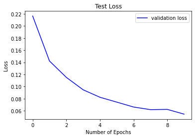
# Plot the loss and accuracy curves for training and validation
plt.plot(history.history['val_loss'], color='b', label='validation loss')
plt.title("Test Loss")
plt.xlabel("Number of Epochs")
plt.ylabel("Loss")
plt.legend()
plt.show()
'''
결과5
'''model.fit() 메서드는 History 오브젝트를 반환합니다. History.history 속성은 연속된 epoch에 걸쳐 학습 손실값과 학습 측정 항목값을 기록하는 딕셔너리 입니다. 적용가능한 경우, 검증 손실값, 검증 측정 항목값을 기록하기도 합니다.
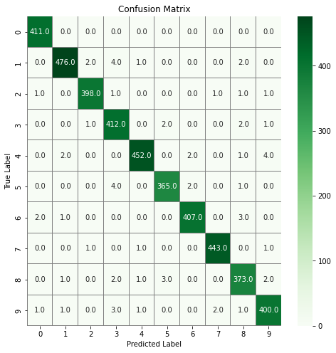
# confusion matrix
import seaborn as sns
# Predict the values from the validation dataset
Y_pred = model.predict(X_val)
# Convert predictions classes to one hot vectors
Y_pred_classes = np.argmax(Y_pred, axis=1)
# Convert validation observations to one hot vectors
Y_true = np.argmax(Y_val, axis=1)
# compute the confusion matrix
confusion_mtx = confusion_matrix(Y_true, Y_pred_classes)
# plot the confusion matrix
f, ax = plt.subplots(figsize=(8, 8))
sns.heatmap(confusion_mtx, annot=True, linewidths=0.01, cmap="Greens", linecolor="gray", fmt='.1f', ax=ax)
plt.xlabel("Predicted Label")
plt.ylabel("True Label")
plt.title("Confusion Matrix")
plt.show()
'''
결과6
'''np.argmax(a, axis=None, out=None)
a = np.arange(6).reshape(2,3) + 10
a
'''
array([[10, 11, 12],
       [13, 14, 15]])
'''
np.argmax(a)
'''
5
'''
np.argmax(a, axis=0)
'''
array([1, 1, 1])
'''
np.argmax(a, axis=1)
'''
array([2, 2])
'''
가장 큰 값의 index를 반환하는데, One-Hot Encoding을 하면 0은 [1, 0, 0, 0, 0, 0, 0, 0, 0, 0]이므로 0이 반환 된다.
sns.heatmap(data, **kwargs)
- annot: 각 cell의 값 표기 유무
참고:
https://whereisend.tistory.com/53
https://tykimos.github.io/2017/03/08/CNN_Getting_Started/
https://blog.naver.com/handuelly/221822938182
'kaggle' 카테고리의 다른 글
| TPSJAN22-01 EDA 필사 (0) | 2022.01.12 |
|---|---|
| Tabular Playground Series - Jan 2022, pycaret 필사 (0) | 2022.01.07 |
| Kaggle Digit Recognizer 필사 (0) | 2021.12.22 |