import numpy as np
import pandas as pd
from keras.models import Sequential
from keras import layers
from keras.layers import BatchNormalization
from keras.layers import Convolution2D, MaxPooling2D
from keras.layers.core import Reshape, Dense, Flatten, Dropout
from sklearn.model_selection import train_test_split
df_train = pd.read_csv('/content/drive/MyDrive/military/mnist/train.csv')
target = df_train[["label"]]
feature = df_train.drop(columns=["label"], axis=1)
x_train, x_test, y_train, y_test = train_test_split(feature, target, test_size=0.25)y_train = pd.get_dummies(y_train.astype(str))
y_test = pd.get_dummies(y_test.astype(str))net = Sequential()
net.add(layers.Dense(510, activation='relu', input_dim=784))
net.add(layers.Dense(100, activation='relu'))
net.add(layers.Dense(75, activation='relu'))
net.add(layers.Dense(60, activation='relu'))
net.add(layers.Dense(50, activation='selu'))
net.add(layers.Dense(25, activation='relu'))
net.add(layers.Dense(20, activation='selu'))
net.add(layers.Dense(15, activation='relu'))
net.add(layers.Dense(10, activation='softmax'))
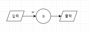
net.compile(optimizer='Adam', loss='categorical_crossentropy', metrics=['accuracy'])Keras에서는 모델을 만드는 방법이 두 가지가 있는데, 그 중 하나가 Sequential 모델이고 순차적으로 레이어 층을 더해주기 때문에 순차 모델이라 불린다. 첫 번째 노드를 보면, 입력이 784, 출력이 510이다.
model.add를 하면 모델 안에 있는 다른 노드들과 연결 된다. Dense 클래스는 입력과 출력을 모두 연결해주는 NN 레이어 노드를 만든다. Dense로 만든 노드는 W, B를 가진다. W는 가중치, B는 편향이다.
model_net = net.fit(x_train, y_train, epochs=10, batch_size=64, validation_split=0.1)
'''
Epoch 1/10
443/443 [==============================] - 5s 9ms/step - loss: 0.7711 - accuracy: 0.7792 - val_loss: 0.3748 - val_accuracy: 0.8962
Epoch 2/10
443/443 [==============================] - 4s 9ms/step - loss: 0.2417 - accuracy: 0.9328 - val_loss: 0.2447 - val_accuracy: 0.9302
Epoch 3/10
..
Epoch 9/10
443/443 [==============================] - 4s 8ms/step - loss: 0.0654 - accuracy: 0.9809 - val_loss: 0.1384 - val_accuracy: 0.9660
Epoch 10/10
443/443 [==============================] - 4s 8ms/step - loss: 0.0608 - accuracy: 0.9828 - val_loss: 0.1849 - val_accuracy: 0.9565
'''
score= net.evaluate(x_test, y_test, batch_size=64)
score
'''
165/165 [==============================] - 1s 4ms/step - loss: 0.1905 - accuracy: 0.9534
[0.190480574965477, 0.9534285664558411]
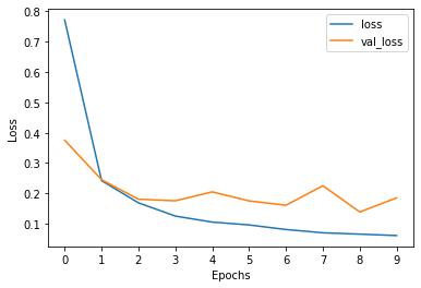
'''import matplotlib.pyplot as plt
pd.DataFrame(model_net.history).loc[:, ['loss', 'val_loss']].plot()
plt.xticks(range(10))
plt.xlabel('Epochs')
plt.ylabel('Loss')
plt.show()
'''
결과1
'''
net.summary()
"""
Model: "sequential_1"
_________________________________________________________________
Layer (type) Output Shape Param #
=================================================================
dense (Dense) (None, 510) 400350
dense_1 (Dense) (None, 100) 51100
dense_2 (Dense) (None, 75) 7575
dense_3 (Dense) (None, 60) 4560
dense_4 (Dense) (None, 50) 3050
dense_5 (Dense) (None, 25) 1275
dense_6 (Dense) (None, 20) 520
dense_7 (Dense) (None, 15) 315
dense_8 (Dense) (None, 10) 160
=================================================================
Total params: 468,905
Trainable params: 468,905
Non-trainable params: 0
_________________________________________________________________
"""model.summary()는 만들어진 모델의 형태를 확인하게 해준다.
Convolution
x_train = x_train.astype('float32')
x_test = x_test.astype('float32')
model = Sequential([
	Reshape((28, 28, 1)),
    Convolution2D(32, (3, 3), activation='relu'),
    Convolution2D(32, (3, 3), activation='relu'),
    MaxPooling2D(),
    Convolution2D(64, (3, 3), activation='relu'),
    Convolution2D(64, (3, 3), activation='relu'),
    MaxPooling2D(),
    Flatten(),
    Dense(512, activation='relu'),
    Dense(200, activation='relu'),
    Dense(150, activation='relu'),
    Dense(100, activation='relu'),
    Dense(75, activation='selu'),
    Dense(50, activation='relu'),
    Dense(25, activation='relu'),
    Dense(10, activation='softmax')
])
tf.keras.layers.Reshape
tf.keras.layers.Reshape( target_shape, **kwargs) 입력을 주어진 모양으로 재구성하는 레이어입니다.
model = tf.keras.Sequential()
model.add(tf.keras.layers.Reshape((3, 4), input_shape=(12,)))
model.output_shape
# (None, 3, 4)
첫 번째 레이어로 사용할 때는 input_shape를 사용해서 들어올 데이터의 크기를 알려주어야합니다. 중간에 쓸 때는 input_shape를 사용하지 않습니다. '-1'차원도 지원합니다.
# also supports shape inference using '-1' as dimension
model.add(tf.keras.layers.Reshape((-1, 2, 2)))
model.output_shape
(None, 3, 2, 2)
tf.keras.layers.Conv2D
tf.keras.layers.Conv2D(
	filters, kernel_size, strides=(1, 1), padding='valid',
    data_format=None, dilation_rate=(1, 1), groups=1, activation=None,
    use_bias=True, kernel_initializer='glorot_uniform',
    bias_initializer='zeros', kernel_regularizer=None,
    bias_regularizer=None, activity_regularizer=None, kernel_constraint=None,
    bias_constraint=None, **kwargs
)
이 레이어는 출력 텐서를 생성하기 위해 레이어 입력과 관련된 컨볼루션 커널을 만듭니다. 이 모델을 첫 번째 레이어로 사용할 경우 data_format="channels_last"에서 키워드 인수 input_shape를 입력해야합니다. 커널은 필터와 같은 말로, 합성곱 계층에서의 가중치에 해당하며 필터를 적용해 유사한 이미지의 영역을 강조하는 특성 맵(feature map)을 출력하여 다음 계층으로 전달한다. filters는 필터의 개수(특징 맵의 개수)로 정수 형태로 입력받는다.
input_shape = (batches_size, rows, cols, channels) > Ouput_shape = (batches_size, rows, cols, channels), 단 이 레이어를 첫 계층으로 사용할 때 input_shape=(row, cols, channels)로 입력해주어야 한다.
return = activation 함수( Conv2D(input, kernel) + bias )
# 입력은 'channels_last'와 배치가 있는 28x28 RGB 이미지입니다.
# 크기는 4입니다.
input_shape = (4, 28, 28, 3)
x = tf.random.normal(input_shape)

# input_shape[1:] => (28, 28, 3)
y = tf.keras.layers.Conv2D(
	2, 3, activation='relu', input_shape=input_shape[1:])(x)
print(y.shape)
# (4, 26, 26, 2)
)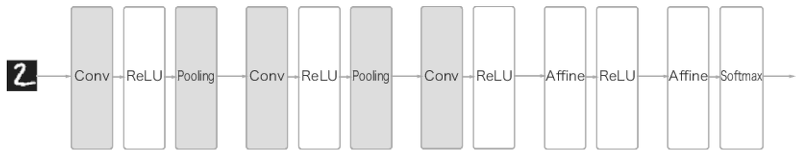
Affine 계층은 순전파 과정에서 수행하는 뉴런에 가중치를 곱하고 편향을 더하는 계층, 즉 행렬의 내적이라고 생각하면 된다.
여기서 텐서란 배열의 집합을 말하는데, 표의 3-tensor 예시는 (3, 2, 2)의 3차원 텐서이다.
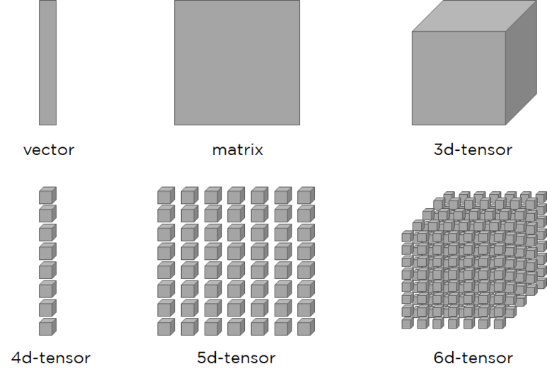
| RANK | TYPE | EXAMPLE |
| 0 | scalar | [1] |
| 1 | vector | [1,1] |
| 2 | matrix | [[1,1],[1,1]] |
| 3 | 3-tensor | [[[1,1],[1,1]],[[1,1],[1,1]],[[1,2],[2,1]]] |
| n | n-tensor |
tf.keras.layers.MaxPooling2D
tf.keras.layers.MaxPool2D(
	pool_size=(2, 2), strides=None, padding='valid', data_format=None,
    **kwargs
)
pool_size는 창의 크기를 지정한 것이고, 창에 포함된 값들 중 최댓값을 샘플링해 다운 샘플링합니다. 창은 각 차원에서 strides 만큼 이동합니다. 'valid'는 padding을 지정하지 않은 결과로 output_shape = (input_shape - pool_size + 1)/(strides)가 됩니다. stride가 (2, 2)일 경우 왼쪽으로 2칸씩 가다가 내려갈 때도 2칸씩 내려간다는 의미이다.
폴링 계층(Pooling Layer)을 사용하는 데는 이미지의 크기를 줄이면서도 데이터 손실을 막기 위해 합성곱 계층에서 strides 값을 1로 지정하는 대신, 폴링 계층을 사용하기도 한다. 또 다른 이유로는 합성곱 계층의 과적합(Overfitting)(융통성 없이 돌아간 사진이나 조금 잘린 사진 등을 인식하지 못하는 등)을 막기 위해 폴링 계층을 사용한다.
Maxpooling은 최댓값을 샘플링하지만, AveragePooling은 평균값을 샘플링한다.
tf.keras.layers.Flatten
입력을 평평하게 합니다. 배치 크기에 영향을 받지 않습니다.
tf.keras.layers.Flatten(
	data_format=None, **kwargs
)
model = tf.keras.Sequential()
model.add(tf.keras.layers.Conv2D(64, 3, 3, input_shape=(3, 32, 32)))
model.output_shape
(None, 1, 10, 64)
model.add(Flatten())
model.output_shape
(None, 640)
model.compile(optimizer='Adam', loss='categorical_crossentropy', metrics=['accuracy'])
con_net = model.fit(x=x_train, y=y_train, batch_size=64, validation_split=0.1, epochs=10)
"""
Epoch 1/10
443/443 [==============================] - 94s 208ms/step - loss: 0.3228 - accuracy: 0.9037 - val_loss: 0.0692 - val_accuracy: 0.9806
Epoch 2/10
443/443 [==============================] - 67s 151ms/step - loss: 0.0699 - accuracy: 0.9797 - val_loss: 0.0840 - val_accuracy: 0.9784
...
Epoch 9/10
443/443 [==============================] - 70s 159ms/step - loss: 0.0223 - accuracy: 0.9946 - val_loss: 0.0471 - val_accuracy: 0.9889
Epoch 10/10
443/443 [==============================] - 66s 150ms/step - loss: 0.0264 - accuracy: 0.9937 - val_loss: 0.0547 - val_accuracy: 0.9895
"""
model.compile()
주요 파라미터
- 손실함수 종류(loss function)
- 훈련 최적화 기법(optimizer)
- 성능 평가 방법(metrics)
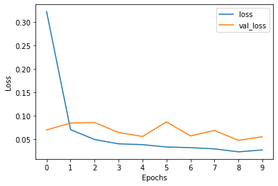
pd.DataFrame(con_net.history).loc[:, ['loss', 'val_loss']].plot()
plt.xticks(range(10))
plt.xlabel('Epochs')
plt.ylabel('Loss')
plt.show()
'''
결과2
'''
y_test = y_test.astype(int)
model.evaluate(x=x_test, y=y_test, batch_size=64)
'''
165/165 [==============================] - 7s 41ms/step - loss: 0.0304 - accuracy: 0.9933
[0.030351318418979645, 0.9933333396911621]
'''
참고 사이트:
https://runebook.dev/ko/docs/tensorflow/keras/layers/flatten
https://dsbook.tistory.com/72?category=780563
https://sdc-james.gitbook.io/onebook/4.-and/5.2./5.2.3.
https://rekt77.tistory.com/102
https://runebook.dev/ko/docs/tensorflow/keras/layers/reshape
'kaggle' 카테고리의 다른 글
| TPSJAN22-01 EDA 필사 (0) | 2022.01.12 |
|---|---|
| Tabular Playground Series - Jan 2022, pycaret 필사 (0) | 2022.01.07 |
| kaggle Digit Recognizer 필사2 (0) | 2021.12.24 |